|
CArl
Code Arlequin / C++ implementation
|
|
CArl
Code Arlequin / C++ implementation
|
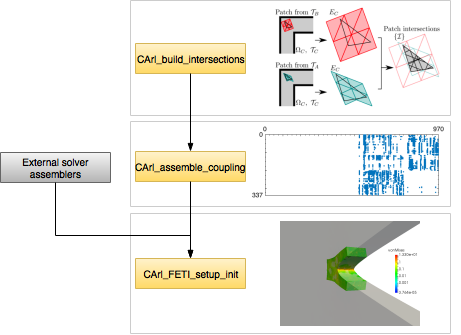
The C++ implementation of the Arlequin method follows the algorithms presented in ref. 1, and it is roughly divided into three parts:
The first two steps are implemented in the CArl_build_intersections and CArl_assemble_coupling, respectivelly. Their corresponding pages contain the documentation of the input parameters.
The coupled system solver uses the FETI method (see ref. 2) to calculate the coupled solutions of the two systems. To allow the usage of external solvers in a non-intrusive way, the implementation is broken down into several CArl_FETI_*** binaries. If the user is using a scheduler program such as PBS, he only has to configure and launch the CArl_FETI_setup_init binary.
If the user is not using a scheduler, the CArl_FETI_setup_init binary will still take care of preparing the other binaries' input files, but the user will have to launch them by hand! Each binary will still return the command that the user has to run, but due to this limitation, the usage of a scheduler is highly recomended. This limitation is due to the fact that mpirun cannot be called recursively in the same shell.
Before calling the coupled system solver, though, the user has to do any preliminary operations involving the external solvers, including preparing their input parameter files. The output of the coupled system solver is a vector in the PETSc binary format.
The figure below presents a workflow for using the C++ version of CArl. The page Examples shows, in detailed steps, how to run a simple test case using external solvers based on the libMesh library. Finally, a more detailed description of the role of each CArl_FETI_*** binaries is presented in the section Implementation of the FETI solver.
All the CArl_FETI_*** binaries take as an input a configuration file though the command line argument -i:
./CArl_FETI_*** -i [input file]
These input files contain parameters such as file paths, output folders, configuration parameters and Boolean flags. They are case-sensitive, and the symbol # is used to comment a single line.
Most of the parameters follow a ParameterName [value] format:
# Cluster scheduler type
ClusterSchedulerType LOCAL

# Path to the base script file
ScriptFile scripts/common_script.sh
Since a space separates the ParameterName and the [value], values containing spaces must be enclosed in `' '`:
# Command used for the external solver for the system A
ExtSolverA 'mpirun -n 4 ./libmesh_solve_linear_system -i '
Boolean flags do not have a [value]. Adding / uncommenting the ParameterName activates the option:
# Use the rigid body modes from the model B?
UseRigidBodyModesB
A description of each file and its parameters can be found at the documentation pages of the corresponding CArl_FETI_*** binaries.
If the matrix of any of the models is ill-conditioned, the FETI solver needs its null space vectors / rigid body modes to work properly. These vectors must be saved in PETSc's binary format. An example of such a model is a linear elastic system under only a traction force. A detailed description of this case is shown in the 3D traction test example.
This section enters in some details of the implementation of the FETI solver, and as such reading the refs. 1 and cpp_usage_note_2 beforehand is highly recommended.
As said above, our implementation of the FETI algortihm is broken down into several CArl_FETI_*** binaries. The "break points" correspond to the operations of the FETI algorithm where the solutions of the external solvers are needed. Before closing, each one of these binaries executes a script which first submits the jobs for the external solver, and then calls the appropriate CArl_FETI_*** binary to continue the algortihm.
This approach allows a non-intrusive usaage of the external solvers: the user only has to worry to save the data to be sent from the CArl_FETI_*** binaries and the external solvers in the appropriate format (see note 3). It also avoids wasting cluster resources with idling jobs.
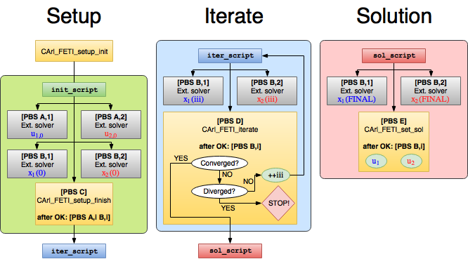
The figure below shows the structure of the FETI solver. It proceeds in the following manner:
init_script.sh, iter_script.sh and sol_script.sh. It then starts the setup of conjugate gradient method (CG) used by the coupled solver to calculate the Lagrange multipliers, and finally executes the init_script.sh script.init_script.sh script runs the external solvers for the uncoupled solutions  (
(  ), and the initial auxiliary vectors
  (if needed). After these solvers are finished, the script launches CArl_FETI_setup_finish.
iter_script.sh.iter_script.sh script runs the external solvers for the  -th auxiliary vectors
  . After these solvers are finished, the script launches CArl_FETI_iterate
iter_script.sh again.sol_script.sh.sol_script.sh runs the external solvers for the final auxiliary vectors  , used to calculate the coupling effects on the models' solutions. After these solvers are finished, the script launches CArl_FETI_set_sol, which assembles and exports the coupled system solutions
  .
.As said above, this process is completely automated if a scheduling software, such as PBS, is used: the user only has to configure and execute the CArl_FETI_setup_init binary. Details about the input parameters of each binary can be found at its documentation page (linked above).
1. T. M. Schlittler, R. Cottereau, Fully scalable implementation of a volume coupling scheme for the modeling of polycrystalline materials, Accepted for publication in Computational Mechanics (2017). DOI 10.1007/s00466-017-1445-9
2. C. Farhat, F. X. Roux, A method of finite element tearing and interconnecting and its parallel solution algorithm, International Journal for Numerical Methods in Engineering 32(6), 1205-1227 (1991). DOI 10.1002/nme.1620320604
3. At the moment, the binaries are capable of reading and writing vectors and matrices in the PETSc binary vectors and matrices. Details of their usage can be found at the documentation of each executable.
 1.8.10
